[Science]   [BAS home]   [Met home]   [Beowulf home]	Antarctic Meteorology

Experiments with different seaices in Hadcm3

Caution: most of the runs here have a "bug" in that they are forced with increasing GHGs, appropriate to their calendar years (2001-201x). This means they have a "drift" which is really not a drift but a response to GHGs imposed on them. Comparison with a control case (yabeo; intended parrallel to aaxzc etc) indicates that the drift is mostly in the tropics and that the seaice is stable here. So I think the results below can be used, but with caution. And of course should be re-run sometime...

The runs used are listed below. All have my version of GR's fix to the IO drag term (ie, negate it to be consistent with FD), and my fix to the scaling-of-drag-and-mass-terms (ie, use WSX not WSX_ICE; scale ISX by aice to give to OI drag; use htrue not h_gbm for mass). None of these runs have the semi-implicit OI drag fix of DC/GR: I believe this to be unnecessary with the fixed OI drag.

Most have p*=27 (my default) and the NP island fix and SSTILT terms on.

Misc notes:

1. My runs are at 32-bit. I find 32/64 makes little difference. But this should be re-checked sometime.
2. Several of these runs died after a few years with an FPE error; usually in ICEFREED (I call it even with EVP just to generate EVP vs FD difference diags, which I then have no time to look at...). Recompiling with -g or somesuch CRUNs OK; so I'm not too worried. But you may be.
3. Remember the MSLP errors in hadcm3 (and the NP probs) when evaluating these runs. Coming soon (hahaha) runs with ERA-forced WSX anomalies.
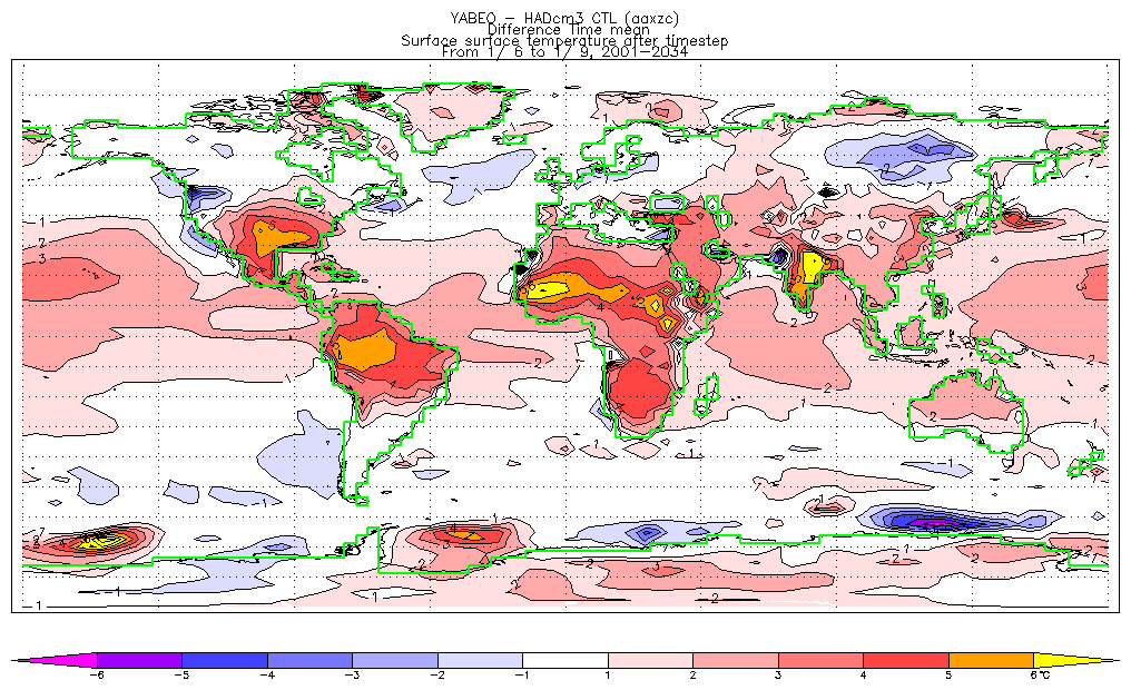
4. I have recently realised that *my* version has unexplained drifts in tropical (but not mid-lat or polar) SSTs. See here for a JJA piccy of a 30-y mean of my SSTs vs HadCM3 100y mean. (This has now been explained: inc GHGs. See caution above).
5. If attempting to model todays ice, shouldn't we start from a 1980's startdump from an appropriate climate change run?

So: the runs:

• Obs (from OMB)
• Hadcm3 (fragment of aaxzc)
• My freedrift (yaben)
• DC's freedrift (abwof)
• My EVP runs (all with DC's NP island fix, and SSTILT turned on):
  • yabpa - p*=0 (similar, one hopes, to FD)
  • yabpb - p*=5k (low value)
  • yabpc - p*=27k (probable best-guess from existing literature)
  • yabpd - p*=100k (too high)
• My version of the "McPhee-like" OI heat flux parametrisation (ie, fluxes as for HadCM3 but multiplied by ice_ocean_shear/tie_point_speed), all with p*=0 (and NP-fix and SSTILT=true), with "tie-points" at:
  • yabph - 5cm/s
  • yabpg - 10cm/s
  • yabpi - 15cm/s
• My dodgy kludge for sub(time,space)gridscale conc-to-depth conversion (p*=27k):
  • yabpd - c2d at (aice-0.5)*0.002 per ocean timestep
  • yabpe/b1 - c2d at (aice-0.5)*0.004
• yabpk - p*=27k, SSTILT *off*

General conclusions

1. Problems seem to be more crudely apparent in the Antarctic than the Arctic. Perhaps this is to be expected, since there is more scope for the dynamics to take effect.
2. Notice the general tendency for the first winter or so to have the most over-extensive ice. Clearly the model is coming into balance with the new sea ice. It is not clear that 10 years is a long enough spin-up. Perhaps I should start the runs from the end of 10 years yabpc?
3. Changing the OI heat flux to McPhee-style seems to help.
4. Overall: several runs improve on "raw" fixed EVP; but only the dodgy c2d is better than hadcm3 OD . McPhee is best plausible scheme so far and should be investigated further, perhaps in conjunction with mild c2d. See plot at end of page.

Go to comparisons

1. Free drift [Summary: FD marginally better than EVP but not by much]
2. EVP [Summary: changing pstar doesn't help too much. No obvious reason not to use 27k.]
3. OI heat flux [Summary: 5 or 10 cm/s looks very promising. Shame they were all run with p*=0]
4. Dubious c2d para [Summary: well, it actually produces what-you-want, ie less ice. Better than HadCM3 areas, in fact. But I forced that in...]
5. Changes to albedo and wind mixing energy [Summary: albedo: removes too much summer ice and too little winter. Wind-dep alb poss for dev]
6. Turn off the sea surface tilt term [Summary: little impact]

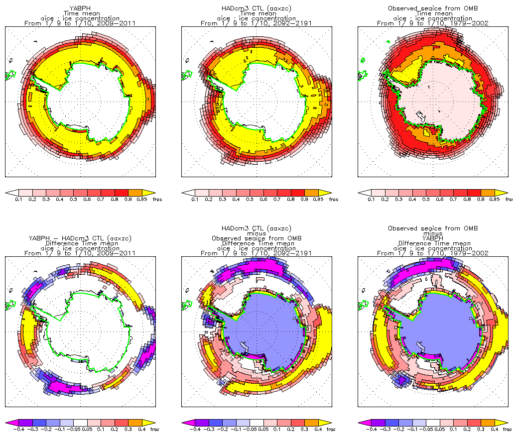
A note on lines and colours

The thick pink line is the long-term mean of the obs. The darker thinner pink inside is each years (well, 1979 on) seaice (from which one may see that the thickess of the pink overestimates natural variability).

My ocean drift (ie hadcm3-a-like) is in black with a white border so you can see it. Hadcm3 10-y fragment is in light blue.

Other line colours vary from plot to plot.

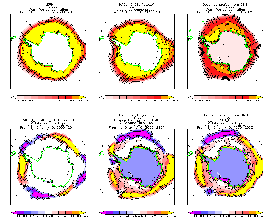
Best Plot

For no especially obvious reason, yabph is more zonally symmetric than hadcm3.

Past last modified: 9/12/2002   /   wmc@bas.ac.uk

© Copyright Natural Environment Research Council - British Antarctic Survey 2002