
|
|
|
| [Science] [BAS home] [Met home] [Beowulf home] | Antarctic Meteorology |
Ideally, the climatology of HADcm3 at BAS should be identical to that at the Hadley Center. But it needs to be run out for some years (more than I have at the momemt) to be seen to be the same above variability.
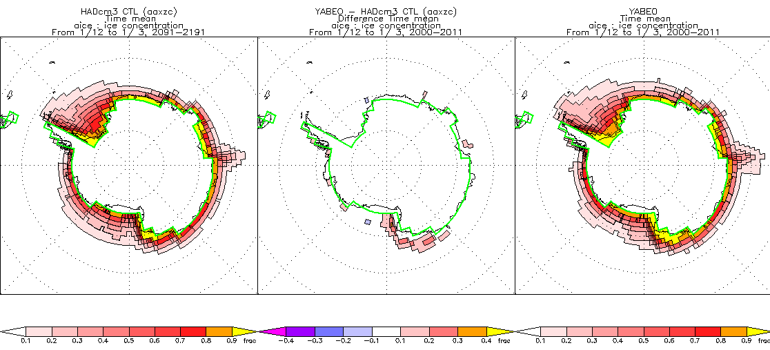
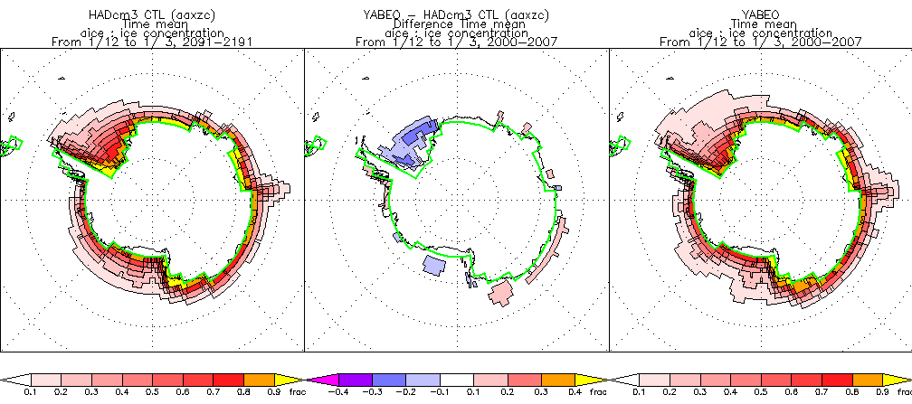
Overview: at first sight, the seaice (which is all I've done so far) looks pretty good, ie the differences from HADcm3 seem small.
The runs here are from HADcm3 (aaxzc, for fans of exactness) and yabeo, a coupled ocean-drift run done at BAS. You can also see yaben, a free-drift run.
AI claims there are problems with denscoef at 32-bit. These are not striking, so far.
There are (perhaps) problems with QT_POS. See yabkb for more on this, which is fixed in yabwb and thus appears to be a problem with the increasing GHG's.
| Sea ice | JJA | DJF | SH | 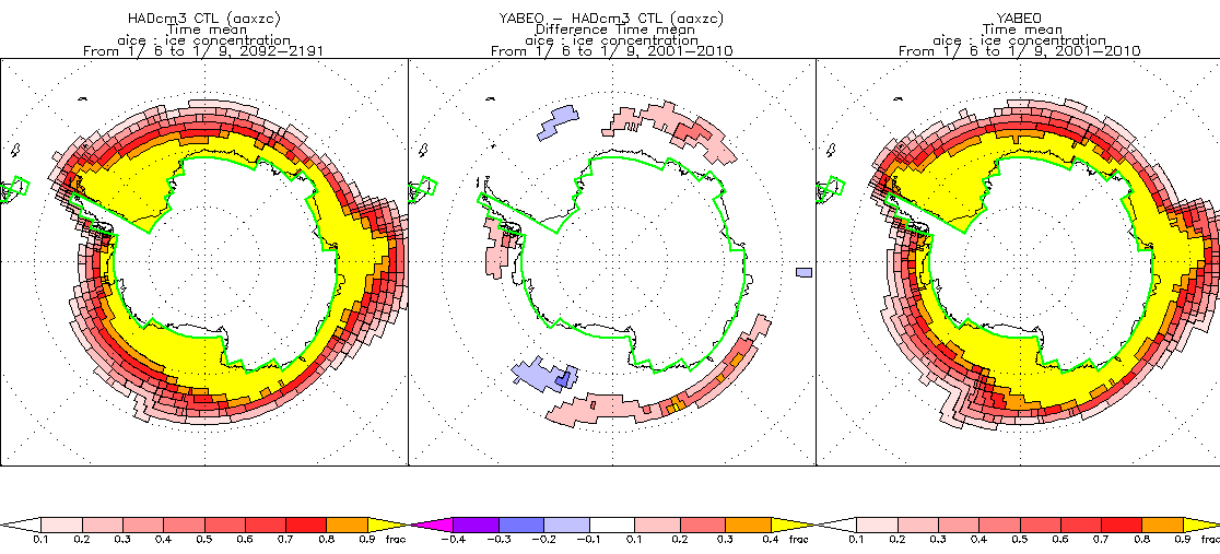 |
 |
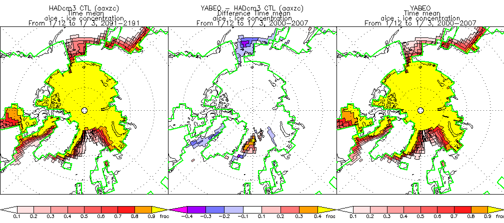
NH | 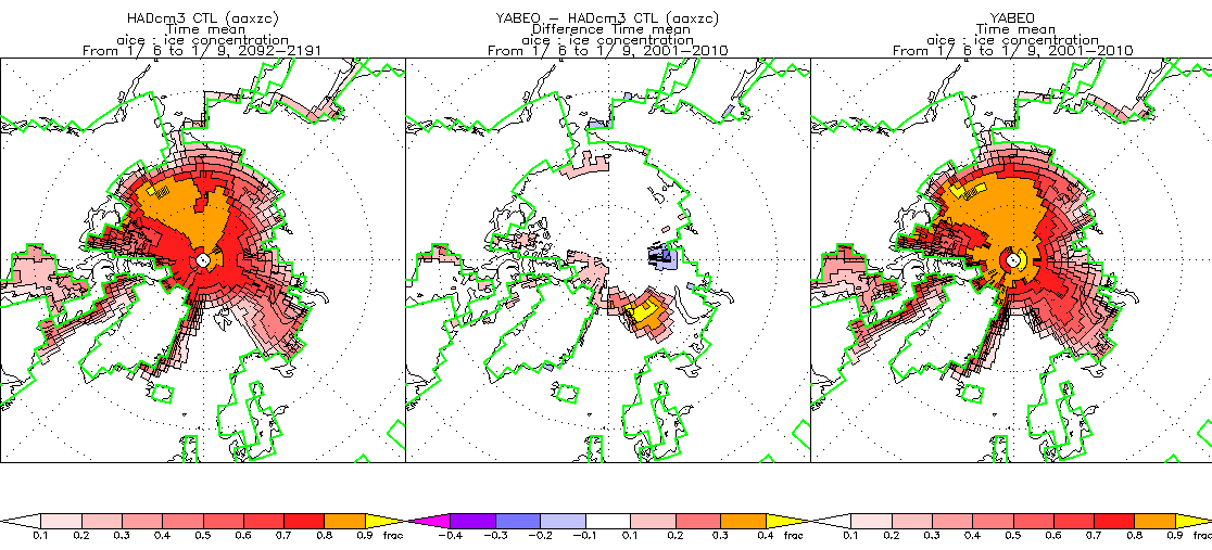 |
 |
there is a blob near Iceland... should I care about that, or is it just variability? Remember also that the 32/64 bit runs start from different start dumps. Hmm... perhaps it would be better for them to start from the *same* one... duhhh.
Lets look by year:
pp_plot,pp_diff(eo32(indgen(9)),ctl3),abc='\year',/notitle,xm=[0,0],ym=[0,0],/nh,col=0
gettwogifs,out='ice-jja-nh-byyear'
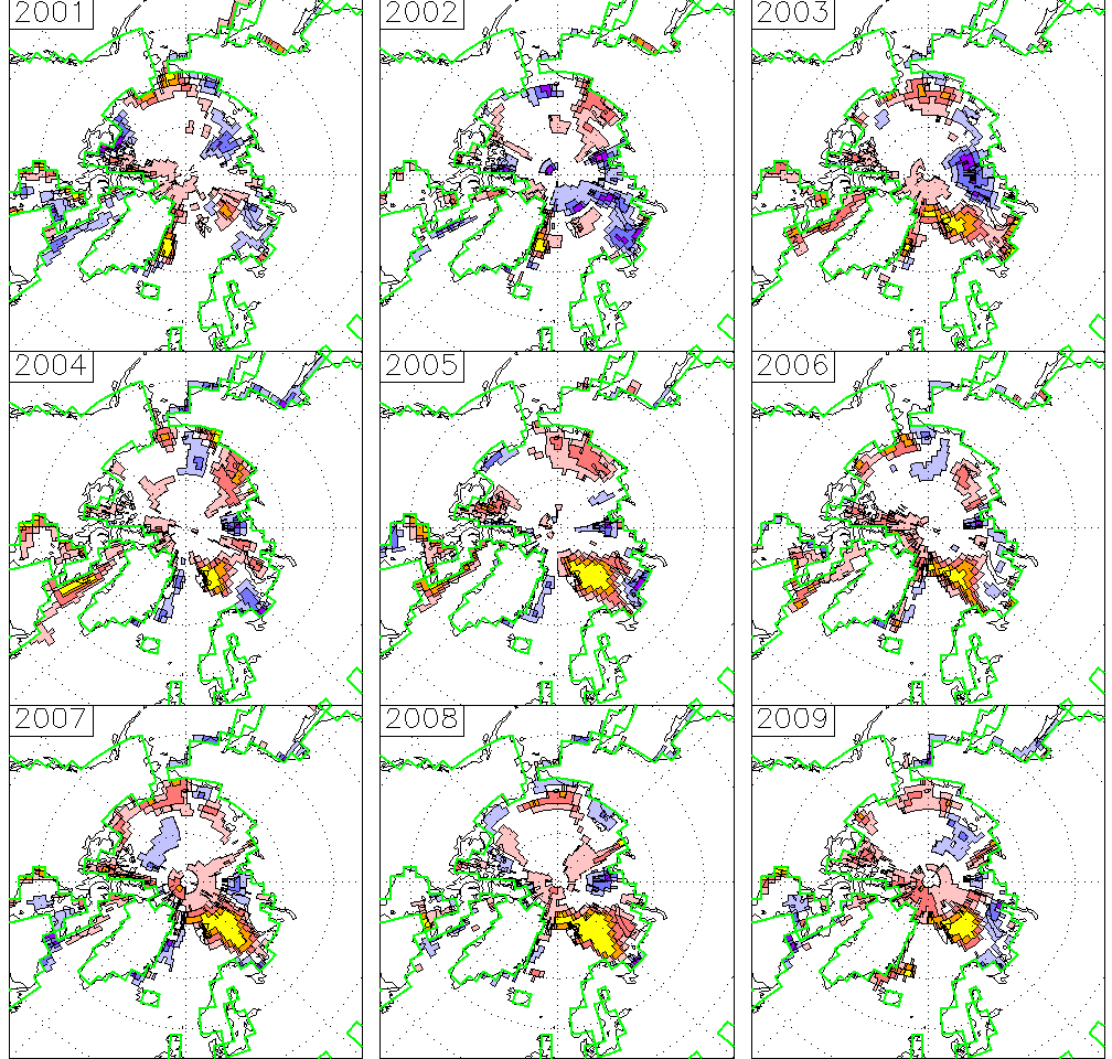
Hmmm... looks suspicious? Could this be the "Denscoef Problem"? Or could it be to do with the "North Pole Problem"?
Now lets look month-by-month at the long-term averages:
a=gm('yabeo/32/x.01m',m=1+indgen(12),var='icec')
b=gm('ctl3/x.01m',m=1+indgen(12),var='icec')
pp_plot,pp_diff(a,b),ster=0,xm=[0,0],ym=[0,0],col=0,/notit,/nh,abc='\mon'
gettwogifs,out='icec.nh.32.by-month'
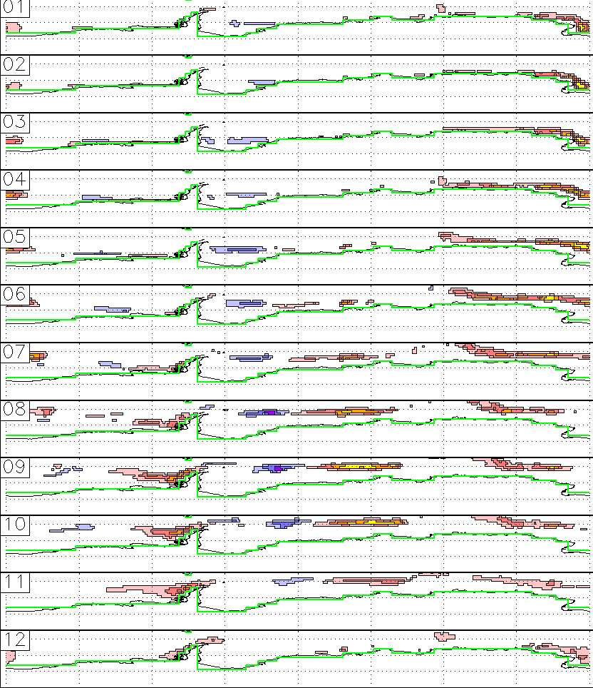
pp_plot,pp_diff(a,b),ster=0,xm=[0,0],ym=[0,0],col=0,/notit,abc='\mon'
gettwogifs,out='icec.sh.32.by-month'
| NH | SH | 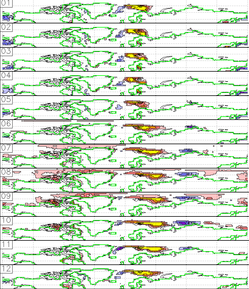 |
 |
@plot_total
gettwogifs,out='total.all'
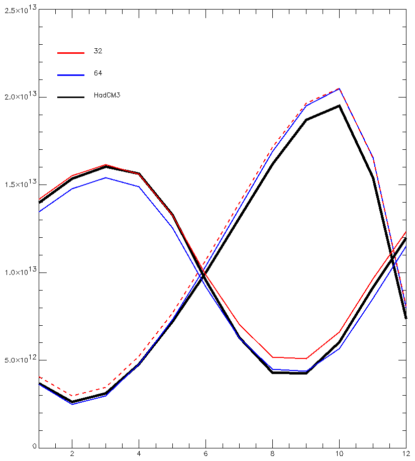
So... both 32 and 64 are pretty close to ctl3 for both hemispheres. Good.
In more detail (but only looking at total area, of course):
| Sea ice | JJA | DJF | SH |  |
 |
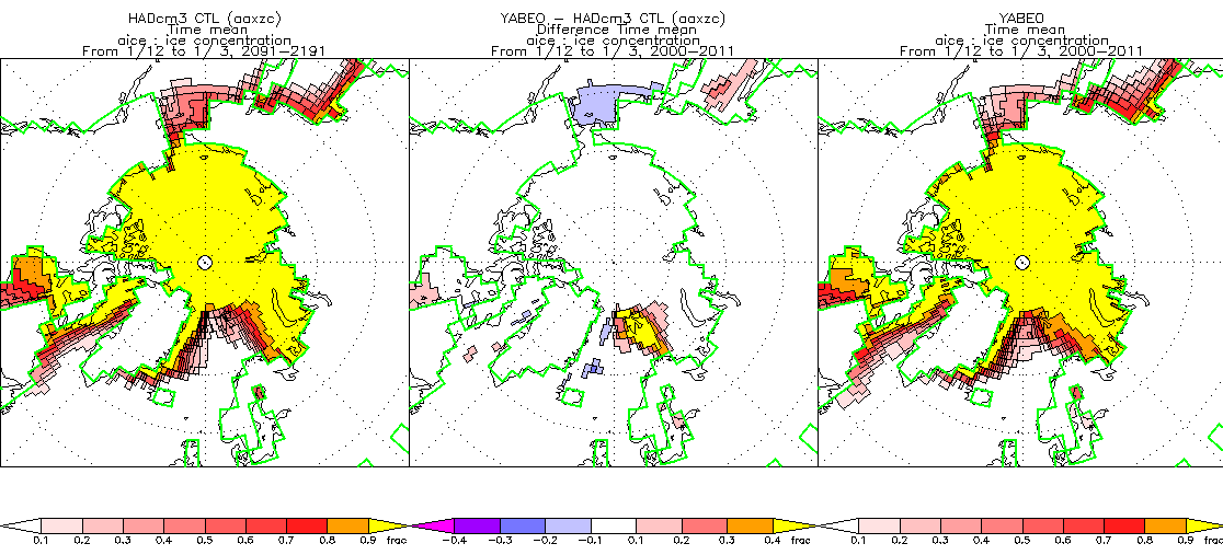
NH | 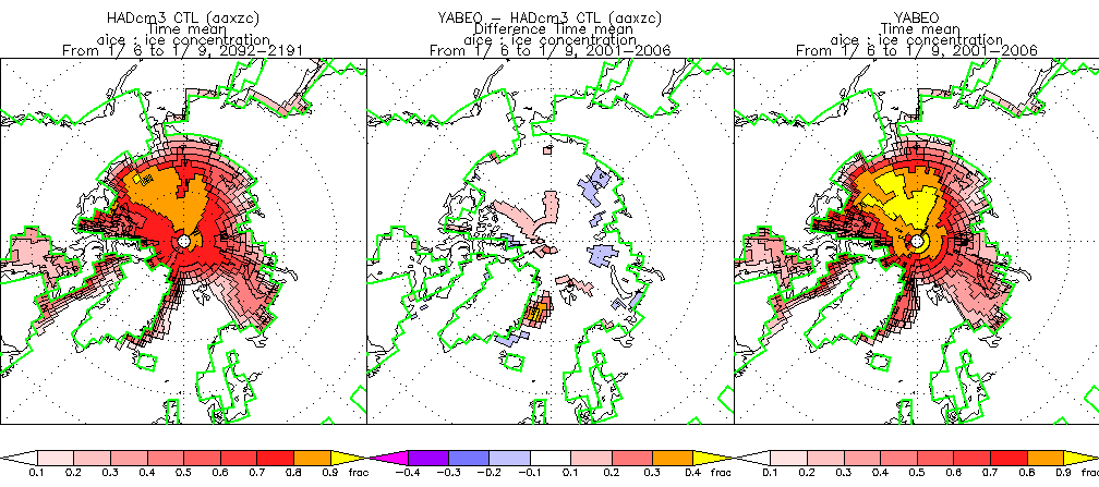 |
 |
Now there is no blob near Iceland... hmmm... at least not year round and not so big... hmm...
Again, look by year:
pp_plot,pp_diff(eo64(indgen(9)),ctl3),abc='\year',/notitle,xm=[0,0],ym=[0,0],/nh,col=0
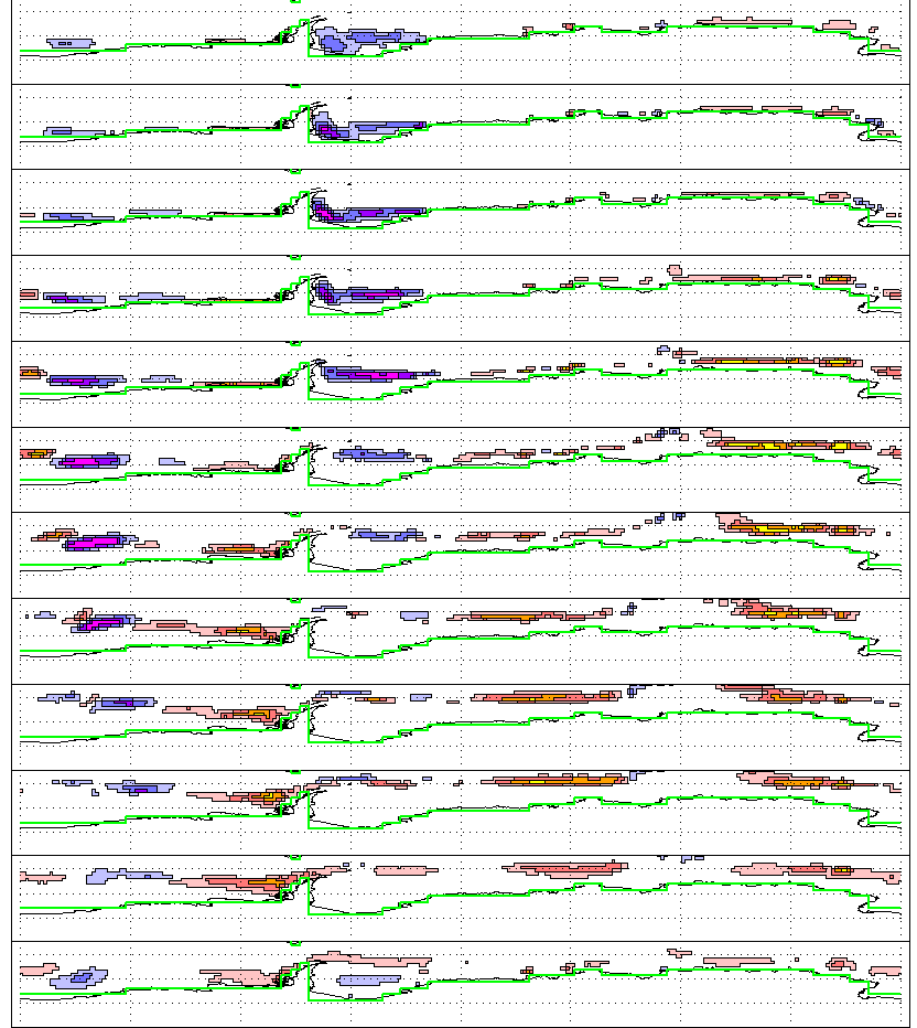
Now lets look month-by-month at the long-term averages:
-missing-
c=gm('yabeo/64/x.01m',m=1+indgen(12),var='icec')
b=gm('ctl3/x.01m',m=1+indgen(12),var='icec')

pp_plot,pp_diff(c,b),ster=0,xm=[0,0],ym=[0,0],col=0,/notit,/nh,abc='\mon'
gettwogifs,out='icec.nh.64.by-month'

pp_plot,pp_diff(c,b),ster=0,xm=[0,0],ym=[0,0],col=0,/notit,abc='\mon'
gettwogifs,out='icec.sh.64.by-month'
| NH | SH | 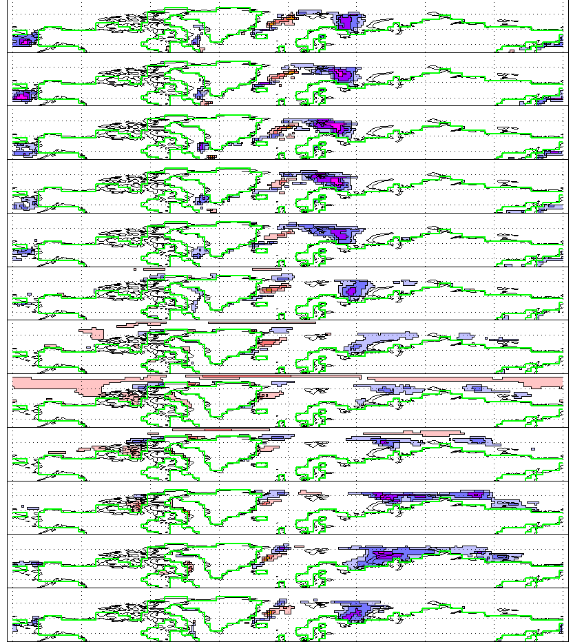 |
 |
| Past last modified: 16/12/2002 / wmc@bas.ac.uk |
© Copyright Natural Environment Research Council - British Antarctic Survey 2002 |