
[Science] [BAS home] [Met home] [Beowulf home]	Antarctic Meteorology

Verification of yabcc - 64 and 32 bit

This is probably obsolete... better to look here for a better go.

This stuff is rather preliminary (only 9 years at present; the 64-bt code is slow...). Read if you like, but with caution.

Note also: these are with correction to the level-by-level constants. See yabba for without.

Note that the IDL code is for my info for regeneration of the piccies.

MSLP

I shall compare against aawei, a job run at the Hadley Center which I believe was a standard HADam3 job.

m=6
run='yabcc'
y=1979+indgen(9)
@../yabba/verify-pstar
gettwogifs,out='pstar_jja'

Produces:

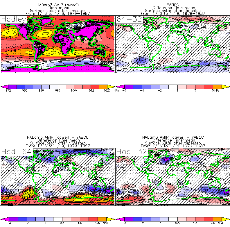
You see: TR: aawei. TL: my jobs, 64 - 32 bit. BR: aawei - 64. BL: aawei - 32.

Note:

that this is pstar.
this is JJA
i have added an attempt at significance testing of the difference drawn on, using t-test of means. Areas unshaded are "significant".

We see: across much of the globe differences are small and non-sig. Excellent. The principal "problem" is around Antarctica :-(.

Meanwhile, back in DJF:

m=12
@../yabba/verify-pstar
gettwogifs,out='pstar_djf'

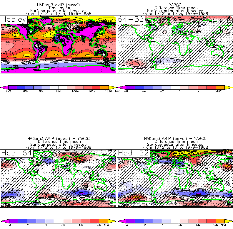
Once again, 32 and 64 bit are very similar. This time, its the NH that shows largest differences between them (winter hemisphere variance is always largest, so this could indicate that the difference is just variability).

Now, however, differences between yabcc and aawei are not huge, as they were in DJF in yabba. Good. Is this chance, or because of fixing the problem with the level by level constants? Note that its still worst in DJF... perhaps the flow is intrinsically harder then?

ACW and SOI

A science result: can we see the Antarctic Circumpolar Wave in yabcc? Yes. OK, its not perfect, but it is there, in 32 and 64-bit versions. Note the flaws common to both. Compare this to yabba.

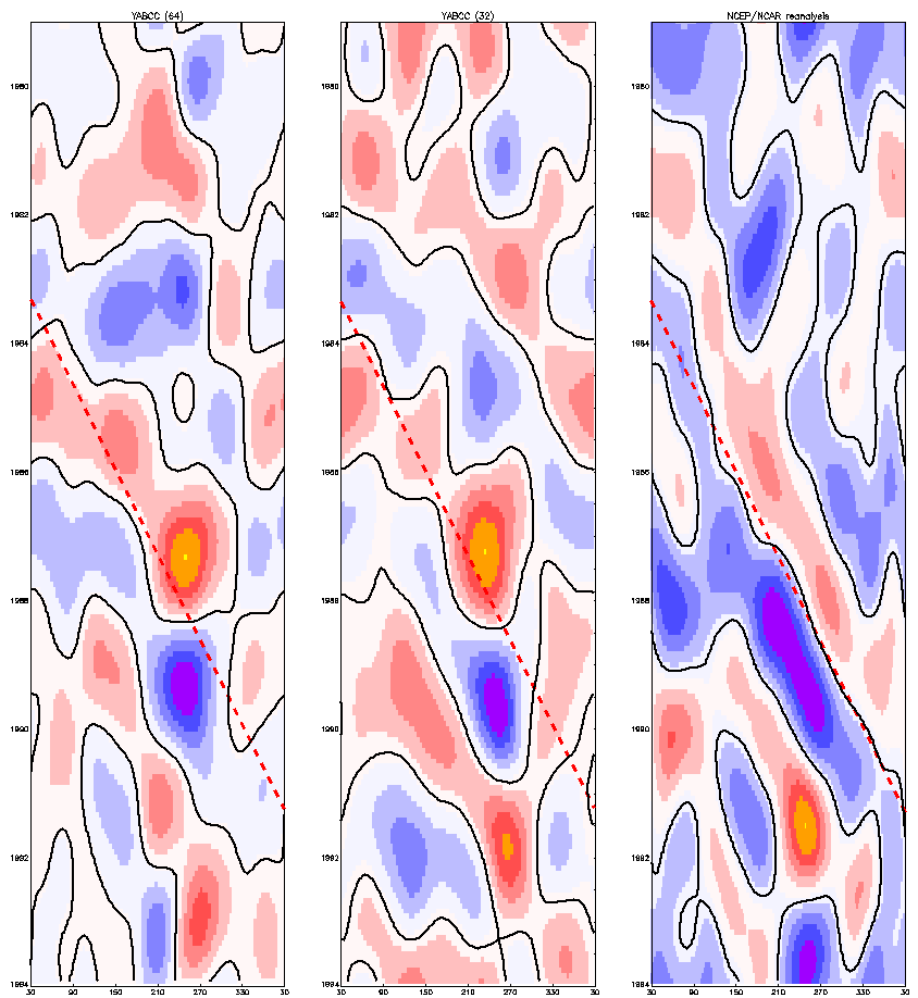
a=gm('yabcc/32/0.01',y=1979+indgen(15),m=1+indgen(12))   
b=gm('yabcc/64/0.01',y=1979+indgen(15),m=1+indgen(12))   
p=gm('NMCclim/0.01',y=1979+indgen(15),m=1+indgen(12))   

hov_acw,b,la=la,xmarg=xm,ymarg=ym,lev=lev,fac=100,f0=f0,ymarg=[2,10],title='YABCC (64)'
hov_acw,a,la=la,xmarg=xm,ymarg=ym,lev=lev,fac=100,f0=f0,ymarg=[2,10],title='YABCC (32)'
hov_acw,p,la=la,xmarg=xm,ymarg=ym,lev=lev,fac=100,f0=f0,ymarg=[2,10],title='NCEP/NCAR reanalysis' 

gettwogifs,out='yabcc-ncep'

How about the SOI?

test_soi,a,p,a1
gettwogifs,out='soi'

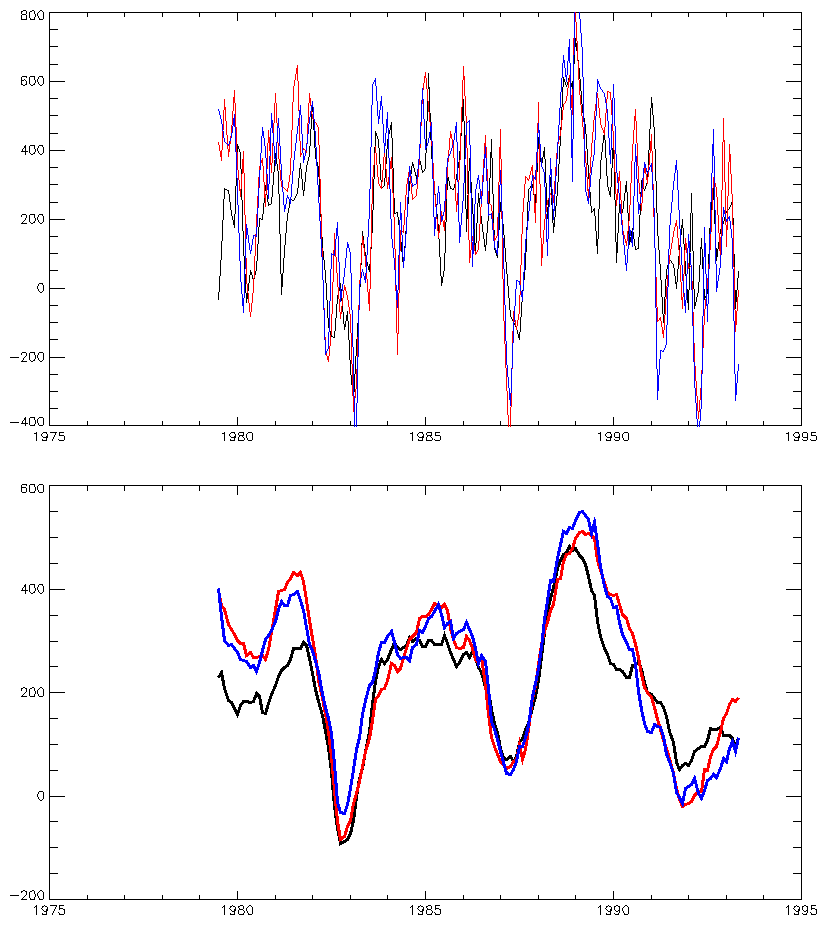
Black: NCEP. Red: 64-bit. Blue: 32-bit.

Past last modified: 9/9/2002 / wmc@bas.ac.uk
© Copyright Natural Environment Research Council - British Antarctic Survey 2001