
[Science] [BAS home] [Met home] [Beowulf home]	Antarctic Meteorology

Verification of yabba - 64 and 32 bit

This stuff is rather preliminary. Read if you like, but with caution.

Note also: these are 20-minute timestep runs *without* the correction to the level-by-level constansts.

Note that the IDL code is for my info for regeneration of the piccies.

MSLP

I shall compare against aawei, a job run at the Hadley Center which I believe was a standard HADam3 job.

m=6
@verify-pstar
gettwogifs,out='pstar_jja'

Produces:

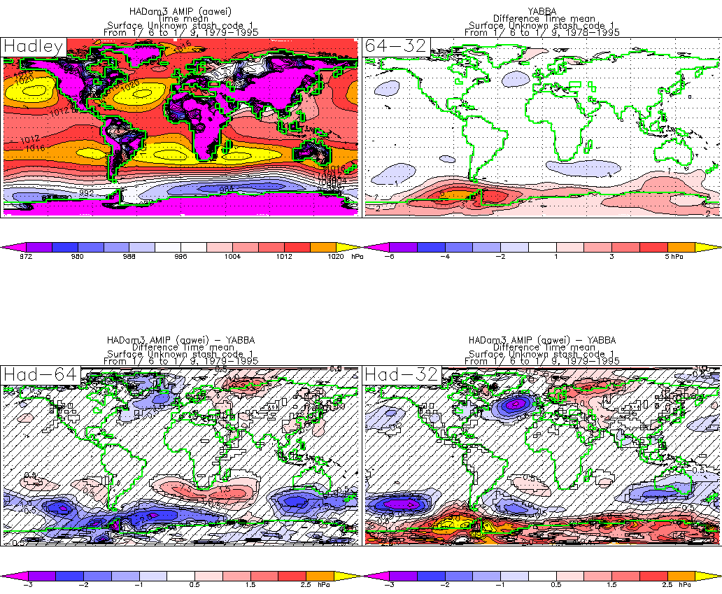
You see: TR: aawei. TL: my jobs, 64 - 32 bit. BR: aawei - 64. BL: aawei - 32.

Note:

that this is pstar.
this is JJA
i have added an attempt at significance testing of the difference drawn on, using t-test of means. Areas unshaded are "significant".

We see: across much of the globe differences are small and non-sig. Excellent. The principal "problem" is around Antarctica :-(.

Meanwhile, back in DJF:

m=12
@verify-pstar
gettwogifs,out='pstar-djf'

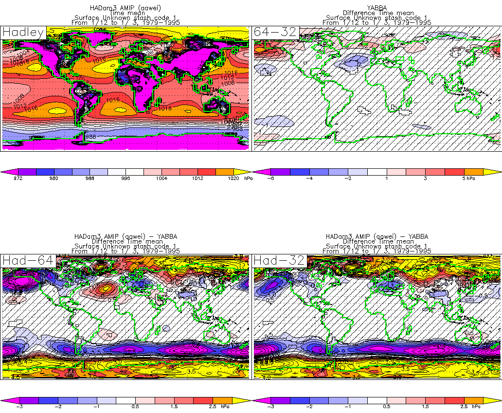
Once again, 32 and 64 bit are very similar. This time, its the NH that shows largest differences between them (winter hemisphere variance is always largest, so this could indicate that the difference is just variability).

Now, however, differences between yabba and aawei are quite large. Odd. Could this be because of the problem with the level by level constants? Possibly: because it gets a lot better in yabcc.

ACW and SOI

A science result: can we see the Antarctic Circumpolar Wave in yabba? Yes. OK, its not perfect, but it is there. These are from the 64-bit version.

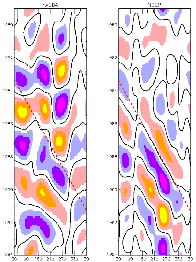
hov_acw,a,la=la,xmarg=xm,ymarg=ym,lev=lev,fac=100,f0=f0,ymarg=[2,10],title='YABBA'
hov_acw,p,la=la,xmarg=xm,ymarg=ym,lev=lev,fac=100,f0=f0,ymarg=[2,10],title='NCEP' 
gettwogifs,out='yabba-ncep'

How about the SOI?

test_soi,a,p,a1
gettwogifs,out='soi'

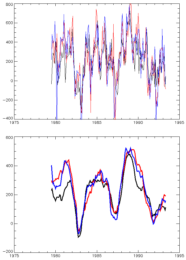
Black: NCEP. Red: 64-bit. Blue: 32-bit.

The stuff below here is a bit older, and involves comparison against HADcm3, and for fewer years.

; 64-bit AMIP (solid)
a=gm('yabba/64/0.03',y=a.lbyr,m=6)  
; 32-bit AMIP (dashed)
b=gm('yabba/32/0.03',y=a.lbyr,m=6)  
; Hadcm3 control from UKMO (aaxzc)
c=pp_scale(gm('ctl3/x.03m',m=6))

a=pp_scale(a)
b=pp_scale(b)

pp_zonal_mean,a,th=3,col=1+indgen(10),yr=[980,1025]
add_key,a.lbyr,indgen(8)+1,th=3                    
pp_zonal_mean,b,th=2,li=2,col=1+indgen(10),/ov          

pp_zonal_mean,c,th=5,/ov

gettwogifs,out='zonal-p'

So... there appears to be (from an 8-year sample) a possible bias between 32 and 64 bit from 60S. But, if anything, the UKMO hadcm3 seems to support the 32 bit!

OTOH, this is a region of large natural variability. It may not be significant.

Also this is a comparison against the HadCM3 control, which (good though it is) has drifted slightly from observed SSTs.

Temperature at 300 hPa

A better test of radiation-type stuff, perhaps?

This time, plot differences from hadcm3 control, since if you plot the things themselves, meridional variation dominates the differences and they all look the same (hey! but thats good!...).

a=gm('yabba/64/0.03',y='all',m=6,var='t.on.p')
b=gm('yabba/32/0.03',y=a.lbyr,m=6,var='t.on.p')
c=gm('ctl3/x.03m',m=6,var='t.on.p',lblev=300)

!p.multi=[0,1,1]                     

pp_zonal_mean,pp_diff(a,c),th=3,col=1+indgen(10),yr=[-3,3]
pp_zonal_mean,pp_diff(b,c),li=2,th=3,col=1+indgen(10),/ov 

add_key,a.lbyr,1+indgen(8),th=3
gettwogifs,out='zonal-t300'

So... on this analysis, 32 and 64 bit are identical.

!p.multi=[0,2,2]

a1=pp_avg(a)
b1=pp_avg(b)

pp_plot,ster=0,la=90,a1,xm=[0,0]
pp_plot,ster=0,la=90,b1,xm=[0,0]
pp_plot,ster=0,la=90,pp_diff(a1,b1),xm=[0,0],lf=0.25
pp_plot,ster=0,la=90,pp_diff(a1,c),xm=[0,0]

gettwogifs,out='t300-diffs'

So: in the average, 64 and 32 bit are indistinguishable (hurrah!). But both show diffs from hadCM3. Perhaps thats OK - should really compare to hadAM3.

Past last modified: 29/4/2002 / wmc@bas.ac.uk
© Copyright Natural Environment Research Council - British Antarctic Survey 2001